Statistical note
Measurement error propagation: your final number is a chain of estimates
Every derived measurement carries the uncertainty of everything that fed into it — calibration, segmentation, background. Propagation is how you compute the combined uncertainty instead of ignoring it.
A reported number like “dry mass = 42 pg” is never a direct readout — it’s the end of a chain: a calibration constant, a segmented cell boundary, a background estimate, a detector noise floor, each contributing its own uncertainty before the final quantity is computed. Error propagation is the practice of tracking how those individual uncertainties combine into the uncertainty of the final number, instead of quietly treating the final measurement as exact.
The idea in one formula
If a final quantity is computed from several noisy inputs, and those inputs are only weakly correlated, first-order (delta-method) propagation says the output variance is approximately:
where is the vector of partial derivatives of with respect to each input (how sensitive the final answer is to each source), and is the covariance matrix of the inputs (how uncertain, and how correlated, each source actually is). In plain terms: a source only matters if the answer is sensitive to it and that source is actually noisy. A calibration constant known to four decimal places contributes almost nothing even if it’s technically an “input”; a segmentation boundary that shifts by a few pixels can dominate the total uncertainty if the final quantity is sensitive to boundary position.
Worked example: dry mass from a QPI measurement
A quantitative phase image converts an optical path difference map into a dry-mass estimate via a calibration constant (the specific refractive increment) and a segmented cell area. Three independent noise sources feed into the final number: phase-measurement noise, calibration-constant uncertainty, and segmentation-boundary uncertainty.
import numpy as np

# Nominal values and their individual uncertainties (illustrative).
phase_signal, phase_sd = 3.2, 0.05      # radians, phase noise
alpha, alpha_sd = 0.0018, 0.00004       # specific refractive increment, mL/g
area, area_sd = 180.0, 6.0              # pixels^2, from segmentation-boundary jitter

def dry_mass(phase, alpha, area):
    return phase * area / alpha         # simplified proportional model

# Finite-difference Jacobian: how sensitive dry_mass is to each input.
eps = 1e-6
base = dry_mass(phase_signal, alpha, area)
d_phase = (dry_mass(phase_signal + eps, alpha, area) - base) / eps
d_alpha = (dry_mass(phase_signal, alpha + eps, area) - base) / eps
d_area  = (dry_mass(phase_signal, alpha, area + eps) - base) / eps

variance = (d_phase * phase_sd) ** 2 + (d_alpha * alpha_sd) ** 2 + (d_area * area_sd) ** 2
print(f"dry mass = {base:.1f} ± {np.sqrt(variance):.1f}")
Running the numbers usually reveals which source actually dominates — often the segmentation boundary, not the calibration constant, even though calibration gets more attention in method write-ups. That’s the practical payoff of propagating error explicitly: it tells you where to invest effort if you want a tighter final number, instead of guessing.
When the simple formula isn’t enough
The delta method above assumes the function is roughly linear near the operating point and that input uncertainties are independent. When a function is strongly nonlinear, or inputs are correlated (a background-estimation error can shift both the numerator and denominator of a ratio together), Monte Carlo propagation is more robust: repeatedly sample each input from its own uncertainty distribution, recompute the final quantity each time, and take the spread of results as the uncertainty. It costs more compute but makes no linearity assumption.
Takeaways
- A final measurement’s uncertainty is a combination of every upstream source’s uncertainty, weighted by how sensitive the final answer is to each one — not just whichever source is easiest to quantify.
- Compute the sensitivity (the Jacobian) before assuming which source dominates; segmentation and boundary effects are underestimated more often than instrument calibration is.
- When the computation is strongly nonlinear or inputs are correlated, prefer Monte Carlo propagation over the linear delta-method approximation.
- Report the propagated uncertainty alongside the estimate itself — a number without it invites treating a noisy quantity as exact.
Continue through the concepts
Related notes
Batch effects and harmonizationSeparate biological differences from acquisition-day, instrument, staining, or processing shifts without erasing real biology.
Image-level versus cell-level inferenceMatch the inferential unit to treatment assignment and biological replication rather than the number of segmented objects.
Evaluating object detection: matching, not just countingWhy detection and counting metrics live or die on the matching rule between predictions and ground truth — and how duplicate detections and missed objects distort the count.
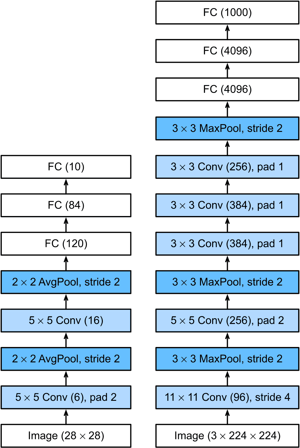 AlexNet: the result that ended the debate about deep learning
How a convolutional network trained on two GPUs cut ImageNet error by a margin large enough to reset computer vision, and why every microscopy segmentation model on this site descends from it.