Hinge loss

A classification metric maps predictions and references to a task-specific utility or loss. Hard-label metrics use a decision threshold; score-based metrics evaluate ranking or probability quality.

Mathematical definition

The central quantity is

$L=mean(max(0,1-y f(x))).$

This expression states what is being counted, averaged, ranked, or compared. Its scale and direction must be interpreted in the context of the data and sampling design.

Compute it in Python

import numpy as np
from sklearn import metrics

y_true = np.array([0, 1, 1, 0, 1, 0])
y_pred = np.array([0, 1, 0, 0, 1, 1])
y_score = np.array([0.1, 0.9, 0.4, 0.2, 0.8, 0.7])
y_prob = y_score
y_true_signed = np.array([-1, 1, 1, -1, 1, -1])
decision_score = np.array([-1.2, 2.1, -0.3, -0.7, 1.5, 0.4])
print(metrics.hinge_loss(y_true_signed, decision_score))

The function is sklearn.metrics.hinge_loss. Inspect its current signature and return object in the official documentation for the version installed in your environment.

Interpretation and cautions

No single metric is universally best. State the positive class, averaging rule, threshold, prevalence, and unit of analysis. Evaluate held-out acquisitions rather than augmented views of training specimens.

A numerical value is not self-interpreting. Compare it with a baseline, uncertainty interval, operational threshold, or competing model, and retain the underlying observations or confusion counts.

Scientific-imaging case study

For margin violations for linear classifiers in a microscopy classifier, inspect per-experiment behavior and the underlying confusion counts before accepting the aggregate score.

Split train, validation, and test data at the specimen or experimental level. Report variability across independent repeats so that the metric describes generalization rather than leakage.

Continue through the concepts

Related notes

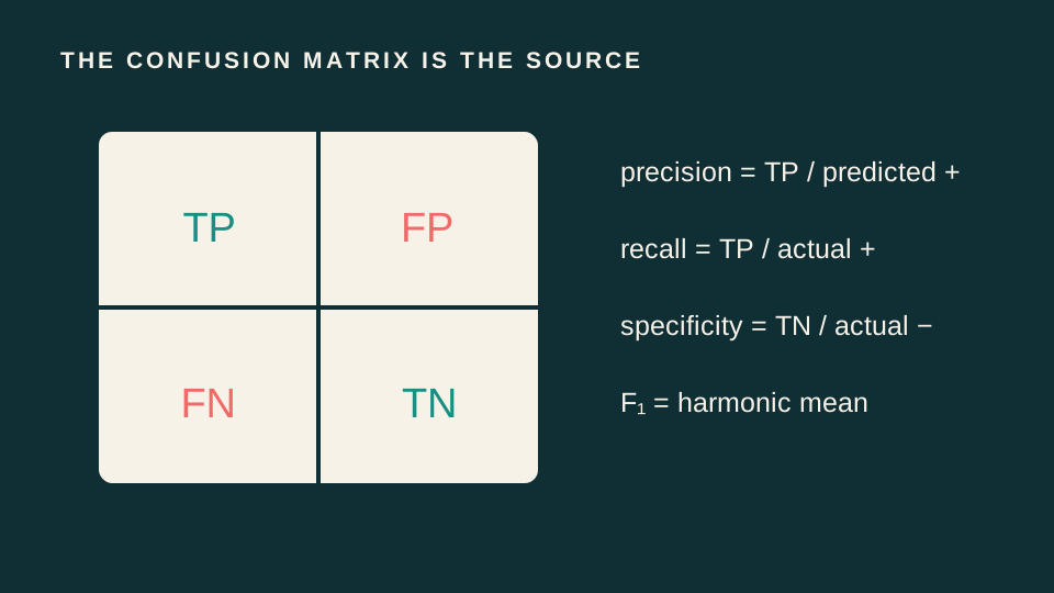
Classification metrics from the confusion matrix

Accuracy, balanced accuracy, precision, recall, specificity, F1, MCC, and choosing metrics under class imbalance.

Accuracy: the simplest classification metric, and its trap

What accuracy actually measures, why it becomes misleading as classes grow imbalanced, and when it's still the right number to report.

Balanced accuracy

Balanced accuracy: theory, interpretation, Python computation, and a scientific-imaging case study.

Precision

Precision: theory, interpretation, Python computation, and a scientific-imaging case study.