Pinball loss for quantile regression

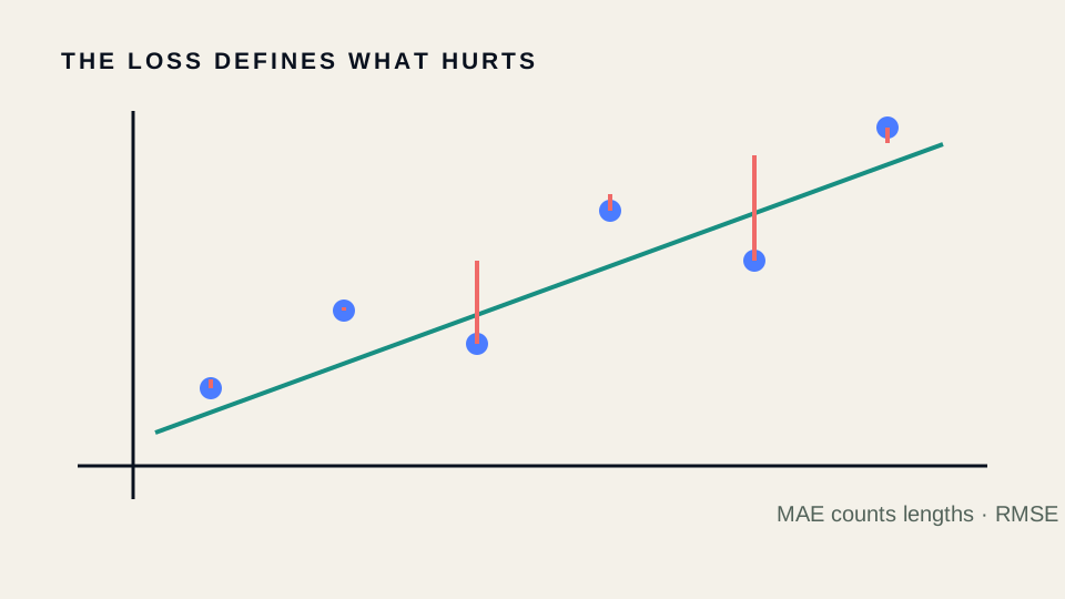
A regression metric defines how residual magnitude, sign, scale, and outcome distribution contribute to model quality. The metric should match the scientific cost of errors.

Mathematical definition

The central quantity is

$L_alpha=e(alpha-I(e<0)).$

This expression states what is being counted, averaged, ranked, or compared. Its scale and direction must be interpreted in the context of the data and sampling design.

Compute it in Python

import numpy as np
from sklearn import metrics

y_true = np.array([1.0, 2.5, 4.0, 7.5, 10.0, 14.0])
y_pred = np.array([1.2, 2.2, 4.8, 7.0, 9.1, 13.2])
print(metrics.mean_pinball_loss(y_true, y_pred, alpha=0.9))

The function is sklearn.metrics.mean_pinball_loss. Inspect its current signature and return object in the official documentation for the version installed in your environment.

Interpretation and cautions

Always examine residual plots and stratified errors. Scale-dependent metrics cannot be compared across outcomes without context; percentage metrics fail near zero; R-squared can be negative on unseen data.

A numerical value is not self-interpreting. Compare it with a baseline, uncertainty interval, operational threshold, or competing model, and retain the underlying observations or confusion counts.

Scientific-imaging case study

For asymmetric quantile prediction error in density-map or QPI prediction, report the score across independent acquisitions and check bias across the target range.

Split train, validation, and test data at the specimen or experimental level. Report variability across independent repeats so that the metric describes generalization rather than leakage.

Continue through the concepts

Related notes

Mean absolute error

Mean absolute error: theory, interpretation, Python computation, and a scientific-imaging case study.

Mean squared error

Mean squared error: theory, interpretation, Python computation, and a scientific-imaging case study.

Root mean squared error

Root mean squared error: theory, interpretation, Python computation, and a scientific-imaging case study.

Mean squared logarithmic error

Mean squared logarithmic error: theory, interpretation, Python computation, and a scientific-imaging case study.