The central limit theorem: why averages become predictable

The central limit theorem (CLT) explains why averages often have approximately normal sampling distributions even when individual observations do not.

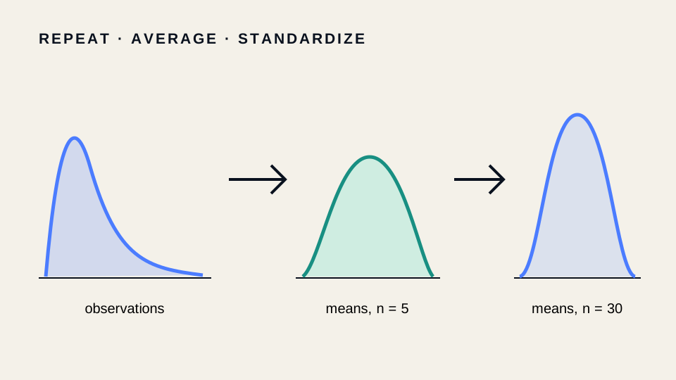
If independent observations share a finite mean and variance, then the standardized sample mean approaches a normal distribution as sample size increases. Its standard error decreases approximately as

$SE(\bar{x})=\frac{\sigma}{\sqrt{n}}.$

import numpy as np

rng = np.random.default_rng(42)
population = rng.lognormal(mean=0.0, sigma=1.1, size=200_000)
for n in (2, 10, 30):
    means = rng.choice(population, size=(10_000, n), replace=True).mean(axis=1)
    print(n, means.mean(), means.std())

What becomes normal?

The theorem concerns the sampling distribution of the mean, not the original data. A large dataset can remain skewed while its mean is estimated with an approximately normal error distribution.

There is no universal magic sample size

Convergence depends on skewness, tail weight, dependence, and the statistic being studied. Heavy-tailed distributions may converge slowly; some distributions do not have finite variance. Clustered biological data also reduce the effective amount of independent information.

Why it matters

The CLT supports many confidence intervals and large-sample tests. It is a reason to understand the sampling process, not permission to ignore it.

Case study: mean dry mass per field

The relevant $n$ may be the number of independent fields, wells, or experiments rather than the number of segmented cells. Correlation inside a field prevents the standard error from shrinking as quickly as the naive $1/\sqrt{\text{cells}}$ calculation suggests.

Continue through the concepts

Related notes

Bayes factors and Bayesian model comparison

Compare marginal evidence carefully, recognising sensitivity to prior scale and the distinction from posterior predictive quality.

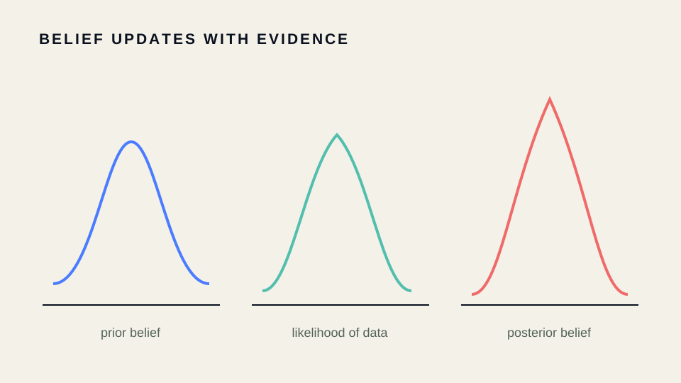
Bayes theorem for statistical inference

Update prior plausibility with data evidence and distinguish posterior probability from a p-value.

Blinding, preregistration, and analysis plans

Reduce conscious and unconscious analytic flexibility by separating confirmatory decisions from observed results.

Credible intervals and highest-density intervals

Summarise posterior uncertainty with direct probability statements while preserving skew or multimodality when important.